Monetary policy only has an effect through changing inflationary expectations.

TO BE NOTED: From Bronte Capital:

"Mr Krugman and Mr Ferguson: a suggested interpretation (very long and ultra wonkish)

This post has an ultra-wonkish warning. Unless you enjoy graduate macroeconomics (soemthing I have never formally done) then you will probably not get many of the short-hand arguments in this post. For that I am sorry.

The main purpose of the post is to provide a basis for discussion amongst button-down modelling macro-economists.

I have just finished reading the blog exchange between Paul Krugman (the Nobel Prize winning economist) and the Niall Ferguson (the historian). As I consider myself a passable economist and a second rate historian this had me enthralled. Moreover, it had me reaching back into the dim recesses of my economics degree for a model. I have one which I will outline below.

The debate is about the meaning of recent kick up in long term interest rates. Mr Ferguson suggesting that it indicates that serious inflation is afoot – or else that the government will shortly have difficulty funding its debt. Mr Krugman has different interpretations – essentially coming down to the stimulus working. For Mr Krugman (the most famous torch bearer for academically rigorous Keynsianism) this debate is central to his world view.

The model needs to deal with the crisis as it is. It needs to be consistent with the facts on the ground of the crisis. It needs to include some kind of difference between real and nominal interest rates (that is some kind of measure of inflationary expectations). And it needs to build into it some kind of rationality for participants in the bond market – otherwise we are assuming away any meaning for the long term interest rate kick up.

It does not need to include a foreign sector or exchange rates because – well – this crisis is remarkably not driven by currency.

The model here – and several of the lemmas – come from Ted Sieper who showed me them during an undergraduate macroeconomics course in 1991. I figure Ted only invented some of it though I do not know who to credit beyond that. Some of it I invented.

I have titled this blog post “a suggested interpretation” after JR Hick’s classic 1937 paper because – well – I use an ISLM model. However it is a very-non-standard ISLM model so I will beg you sit with me through the introduction. I have not written out an ISLM model (or any other macro model) since 1992 – so if this is a little laboured it is because my macroeconomics is rusty. Moreover this model is presented at first away from the zero bound for nominal interest rates. I did not think about the zero bound much when I first looked at this sort of model – because (frankly) it was 1991 and the Great Depression and liquidity traps were an artefact of history. I build in the zero bound in the second part of this note – and that is where the really interesting observations start.

Let’s start.

A standard IS/LM model puts nominal interest rates (i) on the vertical axis and real income (Y) on the horizontal axis. I am going to change it up front (following Sieper) and put both nominal interest rates (i) and real interest rates (r) on the vertical axis and the log of the price level (log p) on the horizontal axis. Distances between nominal and real rates (that is vertical distances) measure expected inflation. For example if expected inflation is 5%, nominal rates are 8% then real rates are 3%.

Distances on the horizontal axis are changes in prices which is the whole point of putting logarithms of the price level on the horizontal axis.

You have to get the axis trick right from the beginning because the rest of my model will not make any sense without it. So just to hammer it home here are the labelled axes. Please do not think this is a standard ISLM model because you will not get anything that follows without noticing this.

Ok, now I am going to put in a Phelps-Friedman supply function. There is a natural level of income (Y) which is a function of real wages (w/p). There is a level of real wages which clears the labour market. However we assume [under most circumstance] that nominal wages (w) are more sticky than the price level (p) at least in the short run. If there is unexpected inflation then the price level is too high, real wages are lower than the “natural level” and there is “excess” employment. If the price level is too low then real wages will be too high – and there will be some unemployment. However as the wages and prices adjust to natural levels we wind up with the natural rate of employment.

Now lets detail an IS curve. In traditional fashion it is a curve which plots equilibrium in the goods market. The demand for goods (again traditionally) is consumption + investment. The supply is income. Consumption (C) is a function of income (Y) which is in turn a function of real wages. Investment (Y) is simply a function of the real interest rate. So here is my IS curve.

Now in the long run my real wage is the market clearing wage and income is fixed. (It’s that Phelps Friedman supply function). That says that Consumption is also fixed and hence the interest rate is fixed at a Wicksellian real interest rate.

The Long Run IS curve is thus horizontal at the Wicksellian Natural Interest Rate (r*). This is pictured below.

This long run curve is labelled IS(L,0) because it is the long run curve in period 0.

It’s a bit strange having a horizontal IS curve – but let us live with that.

Now let’s consider the short run IS curve. In the short run we assume that nominal wages (w) are fixed, but that prices change.

If we increased prices a little we (by assumption above) drop real wages and hence raise income. Both sides of IS curve rise – because consumption also rises with income. But because the marginal propensity to consume is less than one the left hand side would not rise as much as the right hand side. Therefore there would be an imbalance. To get balance back into the goods market (ie to be on the IS Curve) we would need to raise investment. That happens when real rates fall. So – in the short run if we increase prices we have to reduce real interest rates to keep equilibrium in the goods market. The IS curve in the short run thus slopes down. [Thank god for that!]

This is pictured below – with the now usual nomenclature is the long and short run IS curves.

Ok – having got more or less traditional looking IS curves (despite the eclectic choice of axes) let us have a look at Money Market Equilibrium (ie the LM curve). An LM curve would typically have real money demand being equal to real money supply. Money demand (L) is negatively related to nominal interest rates (i) as they represent the cost of holding money and positively related to income (Y). Income – as usual – is a function of the real wage.

Real money supply is just the nominal money supply (m) divided by the price level (p).

Let’s represent that in equation form:

_{As before we consider the shape of a long run and then a short run LM curve.}

In the long run Y is determined (it’s the natural rate). Then as you increase the price level you reduce the real money supply. To get equilibrium in the money market you would also need to reduce the real money demand which you can do by increasing interest rates. The long run LM curve is thus upward sloping. (Again thank God for that.)

Just to rub that in I have drawn another picture.

Now a short run LM curve has another effect when prices rise. Prices rising drive down real wages and up income. This increases money demand – so to get equilibrium in the money market nominal rates would need to rise even further. The short run LM curve is thus steeper than the long run LM curve. I have pictured this below.

Now lets look at a long-run normal time equilibria. Assume that inflation is 5% and always expected to be 5%. As it is a long run equilibria we only need to consider the long run curves. Here is how it will look.

What we have is the LM curve shifting right by 5% per period. The gap between the nominal and real interest rates is 5%. The actual inflation equals the expected inflation.

We can put the short run curves on this – and they look as follows:

OK – now lets model a simple monetary shock. Suppose that there is a sudden and permanent increase in the rate of growth of money supply. We would then expect to be at a long term equilibria say 7% out – and moving out by 7% per year.

We have a new LM curve in period 1 which is to the right of the old one. I have drawn it below and labelled it LM(L,1*) being the shocked curve in period 1.

As we now expect more inflation the gap between nominal interest rates and real interest rates must be larger (that gap is after all inflationary expectations). The new equilibrium will have a sustained 7% gap between nominal and real interest rates. The inflationary expectations will have to equal the realised inflation to that point – so the two lines measured in blue in the above diagram should be of equal length.

Note that the inflationary shock has driven up nominal interest rates in the short run and down real interest rates. The fall in real interest rates causes an increase in income. Monetary change increases short run income. This is entirely consistent with the 80s observed data on monetary “surprises”. When there was a monetary surprise of increased money supply it was associated with increases in nominal interest rates.

I think this is a minimal IS LM model with a reasonable distinction between nominal and real interest rates and a reasonable model of a rational bond market.

Now I need to make an observation which was first made to me by Ted Sieper. I have here a model with rational expectations, a Phelps Friedman expectations determined supply curve and whoa – monetary policy has economic effects. One guy called Robert Lucas Jnr won a Nobel Prize and in part his citation referred to his (definitely faulty) proof that such a thing was impossible. That is the famous so-called “Policy Irrelevance Proposition” (PIP). Well here is the counter example. And if you go look at any proof of the PIP you will find that they either assumed no distinction between nominal and real interest rates or they assumed a vertical LM curve. No – I am not kidding. One of Lucas’s most famous results is bunkum based on faulty maths.

And I do not mean to harp on about it but Lucas’s faulty result poisoned what I think is a very productive well in macroeconomics. Lucas “proved” that rational expectations and an expectations adjusted vertical supply curve made monetary policy irrelevant. However when you looked out the window central banks were clearly using monetary policy to some effect – hence everyone concluded that rational expectations is a bad modelling tool and dumped it.

But the Lucas proof was faulty. There was no reason to dump rational expectations due to the lack of correlation between central bank action and Lucas’s theory. And we have lost the use of a very neat – and quite natural assumption in many macro models.

I need to say this because – as a simplifying assumption I am arguing in this post that the bond market is more or less rational when it is repricing the long end of the curve. [If the argument between Krugman and Ferguson comes down to one side arguing the bond market is wrong or irrational then we are truly lost…] So can all the Keynsians out there not get really annoyed when I use a rational expectations hypothesis – please… Just accept that Lucas's result is wrong...

Moreover – and it is important to observe this – monetary policy again becomes irrelevant whenever the LM curve is vertical. And guess what – the LM curve becomes vertical at the zero bound to inflation – and so we have the standard (but usually faulty) result. But I guess I should model that more formally… as in this model unfortunately the curve becomes horizontal… it does not matter how far or fast prices are falling – nominal rates don’t go below zero…

Embedding the zero bound in this model

It is commonly observed that nominal interest rates cannot rationally stay below zero. The LM curves I drew in the models above have some very strange properties at the zero bound.

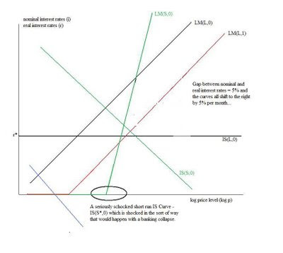
I quite purposely did not have any of my curves (IS or LM) above touch the zero nominal interest rate point – but lets do it now. Here is the long run inflationary equibria curve from above redrawn with the short run LM curve actually touching zero. The rates can’t go below zero – so it does not matter how far prices fall you can’t get negative nominal interest rates… the LM curves go horizontal when nominal interest rates hit zero.

If we are being formal (dotting i’s, crossing t’s, button down macro modelling as Mr Krugman advocates every now and again) we should note that there is – in the short run – some point on this LM curve whereby price levels can’t go any lower without there being deflation. Of course that point is dependent on the previously stable level of inflation – a point that would be moving right every period. Sorry I am getting little beyond my ability to do simple sketches. But I suspect the LM Curve has a period in which it is vertical to the zero until it just becomes as drawn above. Can we ignore this until someone comes up with a better modelling idea?

Now lets seriously shock the IS curve – the sort of shock that makes the zero bound operational – which is for instance what might happen if the banking system collapses…

Ok – now here we are – and its pretty clear that fiscal policy is just effective – because it moves the IS curve right. A move of the IS curve to the right means less deflation is necessary and real wages are less out of kilt.

Monetary policy only has an effect through changing inflationary expectations. If you can induce inflationary expectations then you will need to find a gap between the IS curve and the LM curve such that the gap equals the inflationary expectations. Do that and you will wind up with a very sharply negative real rate of interest.

And you can get there only by say inducing 5% continuous inflationary expectations.

However there is a real problem here – which is that you need to induce inflationary expectations in an environment of falling nominal wages and falling prices – which is tricky to say the least.

You can do it by credibly promising to be reckless (Krugman, Hempton helicopter post). But you can’t do it by being responsible.

Then there is the question as to how reckless you need to promise to be…

If the IS curve has any reasonable slope you need to be massively reckless credibly.

If you do only small changes in money supply then you remain stuck at the zero bound – you do not credibly induce inflation and hence the monetary policy is irrelevant.

Strange result – policy irrelevance holds for small but not big changes in money conditions… and it holds ONLY if you change expectations…

Short summary…

At this point I am coming out at Krugman’s side of the argument – and I think if we model multiple periods we are firmly on Krugman’s side as the yield curve flattens above zero – which is what happened last week.

If anyone wants to do the rest of buttoning this down I will be a keen critic. However the PhD in economics did not ever beckon. I am doing the funds management thing instead...

Oh and if one of those button-down macro-modelling economists can do it thoroughly I would love to put in an external sector. I am trying to understand Spain.

John

Posted by John Hempton "