Significance
Like the Prisoner's Dilemma, this game presents a conflict between self-interest and mutual benefit. If it could be enforced, both players would prefer that they both cooperate throughout the entire game. However, a player's self-interest or players' distrust can interfere and create a situation where both do worse than if they had blindly cooperated. Although the Prisoner's Dilemma has received substantial attention for this fact, the Centipede Game has received relatively less.
Additionally, Binmore (2005) has argued that some real-world situations can be described by the Centipede game. One example he presents is the exchange of goods between parties that distrust each other. Another example Binmore likens to the Centipede game is the mating behavior of an hermaphroditic sea bass which take turns exchanging eggs to fertilize. In these cases, we find cooperation to be abundant.
Since the payoffs for some amount of cooperation in the Centipede game are so much larger than immediate defection, the "rational" solutions given by backward induction can seem paradoxical. This, coupled with the fact that experimental subjects regularly cooperate in the Centipede game has prompted debate over the usefulness of the idealizations involved in the backward induction solutions, see Aumann (1995, 1996) and Binmore (1996).
Centipede Game |
| The centipede game was first introduced by Rosenthal (1982) and has subsequently been studied by Binmore(1987), Kreps (1990) Reny (1988) and many others in different modified forms. The original version of the game consisted of a sequence of a hundred moves (hence the name centipede) with linearly increasing payoffs. |
 |
| Description |
| The centipede game is an extensive-form game in which two players alternately get a chance to take the larger portion of a contiually increasing pile of money. As soon as a player takes, the game ends with that player getting the larger portion of the pile while the other player gets the smaller portion. Passing strictly decreases a player?s payoff if the opponent takes on the next move. If the opponent also passes, the two players are faced with the same choice situation with reversed roles and increased payoffs. The game has a finite number of moves which is known in advance to both players. |
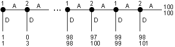
| In the above diagram, a 1 at a black circle ("decision node") denotes a decision opportunity for player 1. A 2 at a decision node tells us that person 2 can make a decision here. The top number at the end of each vertical line is a payoff for player 1 and the bottom number is a payoff for player 2.Player 1 has the first move: if she chooses D, both players get 1; if she chooses A, the opportunity to make a decision passes to player 2. Player 2 has the second move: if he chooses D, player 1 gets payoff of D and he gets 3; if he chooses A, the opportunity to make a decision passes to player 1. And so on to the end of the game tree. If both players always choose A, they both receive payoff of 100 at the end of the game tree. |
| Theoretical Predictions |
| We have just observed that both players receive payoff of 100 if both players always choose A rather than D. Note also that both players receive payoff of 1 if player 1 chooses D on his first move. |
| Typical Experimental Results |
| Studying actual behaviour in different versions ( a four move, six move, and high payoff versions) of the centipede game, McKelvey and Palfrey (1992) found that subjects rarely followed the theoretical predictions. In fact in only 7% of the four-move games, 1% of the six-move games, and 15% of the high payoff games did the first player choose to take on the first move. Similar results were reported by Nagel and Tang (1998). |
| Possible Explanations of "Irrational" Behavior |
| There are two types of explanation to account for the divergence. The first assumes that the subject pool contains a certain proportion of altruists who place a positive weight in their utililty function on the payoff of their opponent. Also to the extent that selfish players believe that there is some probability that other players are altruistics, they have an incentive to mimic altruistic behaviour by passing. The second explanation considers the possibility of action errors. Errors in action, or ?noisy? play, may result from subjects experimenting with different strategies. Or simply from subjects pressing the wrong key. |
| Available Software |
| More Discussions on Variants of the Centipede Game |
| Binmore,K. & McCarthy,J. & Ponti,G. & ..., (1999). "A backward induction experiment," Working papers 34, University of Wisconsin Madison - Social Systems |
| References |
| R.McKelvey and T.Palfrey (1992) ? An experimental study of the centipede game,? Econometrica 60 |
| |
Page source: http://www.econport.org/econport/request?page=man_gametheory_exp_centipede |
Rationality and Game Theory
The discrepancy between the predictions that game theory makes for the way to play the centipede game and what happens in actual practice has created a torrent of research...Joseph Malkevitch
York College (CUNY)
malkevitch at york.cuny.edu ![]()
Introduction
If you were offered $1000, no strings attached, you would probably take the money. And run? If the amount were $10,000 rather than $1000, again, no strings attached, you would probably take the money, and run even faster. However, if you saw a $100 bill lying on the street, and your back had been giving you agonizing pain recently, though currently you were in no pain, you might not bend over to pick it up. Certainly for a quarter (25 cents) it would not be worth it to stoop over. In explaining and offering advice about economic behavior, economists and mathematicians invoke arguments about "rational" behavior to explain what actions people should take. However, as the example above shows, if the decision maker has more information (the state of her back) than the observer, then the behavior observed may be different from the behavior expected.
The Theory of Games, pioneered by the mathematician John Von Neumann (1903-1957)

and the economist Oskar Morganstern (1902-1976),

offers a variety of thought-provoking examples where the difference between the behavior that logic dictates and the behavior actually seen are worlds apart. Thus, Game Theory offers mathematicians, psychologists, political scientists, philosophers, economists, and other scholars an exciting playground for exploring fascinating ideas and a tool for probing a wide variety of problems that are at the core of their disciplines. If one views game theory from a mathematical modeling point of view, where parts of game theory are used to provide a representation for behavior in the "real world," then experiments involving games offer not only a way to improve our insights into human behavior but also a way to develop new approaches and ideas for game theory itself.
Those who are familiar with the theory of games may wish to skim the next section which deals with some relatively well known aspects of game theory. The goal of this preliminary material is to serve as a contrast between what "standard" game theory wisdom suggests about certain games and the way these games are played in practice.
Game Theory: The Basics
Game theory has grown into a complex and multi-branched subject. The basic idea is that one has a group of people (usually referred to as players) who are interacting with each other with some conflict the group desires to resolve. For simplicity, let us consider only two people (countries or companies) as players. Depending on the actions or decisions that are taken by the players, different "payoffs" will accrue to the two people involved. We will assume that the games involved are games of perfect information. This means that each player knows exactly what actions are open to him/her and to his/her opponent. It is also assumed that the payoffs to each player are known and what the value of each payoff is. The games we are interested in here typically arise in daily life, economics and political science (law), in contrast to games such as Nim, Dots and Boxes, and Hackenbush, which are sometimes called combinatorial games. The examples below give the range of conflict situations that game theory illuminates.
Situation 1:
A husband and wife are trying to decide what do on Friday night. The husband would like to see a movie but the wife would like to go to the opera.
Situation 2:
Country X has threatened to test a newly developed nuclear weapon underground and Country Y is upset about the possibility.
Situation 3:
Two children simultaneously flash either two fingers or one finger. If the sum is even, each child wins a dime; if the sum is odd, each child loses a dime.
Situation 4:
Two competing electronic stores must decide whether to use television advertising during the week before the Thanksgiving holiday.
These situations show a small sample of various degrees of seriousness of consequences to the players involved and although only two people (entities) are mentioned, there are often other "parties" affected by the decisions made by players in a game. For example, for the nuclear testing situation, the whole world runs the risk of having radiation released into the atmosphere if something goes wrong with the underground test.
Situations of these kinds may occur only once or may be repeated often under more or less the same circumstances. Sometimes the players may be able to communicate with each other about what actions to take, but in other situations the players interact more or less independently of each other. Even if the players can communicate and reach agreements about how to act when playing the game, there is not always a guarantee that one or both players might not break a "treaty" that they have agreed upon. Sometimes the players may be strangers to each other whereas in other cases they may know each other well. When players do know each other, they might know what their respective values might be as well as the way they think about situations involved in the game. However, even in the case of playing against a stranger, the players may be governed in their actions by their views about fairness, sympathy, and altruism.
When players interact in games of this kind, they may look at the outcomes from the play of the game in complex ways. In some games there is money that changes hands in the game. However, in many cases the outcomes may be measurable on several scales. Thus, for a couple deciding which event to attend on a Friday evening, there may be monetary implications to the outcome (movies are typically cheaper to attend than operas) but also "satisfaction" outcomes. Psychologists and economists, together with mathematicians, have developed theories of "utility" which attempt to allow a player of a game to assign a single number, called a utility, to the outcome that the player receives from a game (or more generally from making some decision). The main idea is that if action A is preferred to action B, then the utility assigned to A should be higher than the utility assigned to B. However, it is well known that in expressing preference humans are not always consistent. Thus, John might prefer apples to bananas, bananas to cherries, but cherries to apples. Some people, when this "intransitivity" of preference is pointed out to them will "correct" their stated preferences; other people will stand by what they have said. This can be because there is no single underlying scale on which the fruit are being judged by this person, which means that when expressing a preference, a person is balancing complex views about the fruits. Thus, when such "cyclic" preferences exist, it will not be possible to assign a number to each of the fruits so that one fruit is preferred to the other when the number assigned to it is higher.
This brief discussion should suggest that "utility theory" is a fascinating and complex subject. Thus, a rich and a poor person would look at the same sum of money that might change hands in a game quite differently. For our purposes let us pretend that the players are able to evaluate for themselves how to measure the outcomes of the game on some scale of utilities. These outcomes of the game arise from the players making a choice among actions that are available to them. An action on the part of each player leads to an outcome. Sometimes the utilities associated with an outcome will be known to both of the players and sometimes they won't. We will also assume that given a choice of a higher versus lower numerical payoff, both players will always select the higher payoff.
It will be convenient to refer to the two players involved in a game as Row and Column. I will use female pronouns for Row and male pronouns for Column. How can we record the actions available to the players of a game? One method is to use a "tree diagram" (graph) where the vertices (sometimes called nodes) of the tree show alternative choices for the player whose move is represented by being at this node. In the simplest case trees are used to merely show alternative actions for the players, but they can also be used to display what information is available to the players at the times choices might be made. Thus, a player's opponent may or may not know what choices an opponent might have at a tree node. When the "moves" and payoffs for a game are displayed in this form, the game is said to be described in "extensive form." A very simple example is displayed below (Figure 1). In the diagram shown, the 1-valent vertices of the tree, or leaves of the tree, are labeled with pairs (r, c) which indicate the payoff to row and column, respectively. Thus, if Row plays her choice II and Column plays his choice 1, then Row receives -$8 and Column receives $8. This can be interpreted to mean that Row pays Column $8.
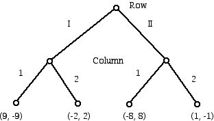
Figure 1
The "extensive form" of this game can be displayed more compactly, and in many respects more clearly (though as previously noted with a loss of generality), if the results are displayed in "normal form." This is done with a matrix, showing Row's choices in the rows of the matrix and Column's choices in the columns of the matrix, as in Figure 2. The payoffs again are displayed as pairs and the Row player's payoff is indicated first in each pair. The way this game is played is that without communicating, the two players choose one of the two actions indicated. For Row this means picking Row I or Row II while for column it means selecting either Column 1 or Column 2. You can think of each of the players as writing either I or II on a piece of paper by Row, and 1 or 2 on a piece of paper by Column, and handing their choice to a "judge." This person then affirms the payoff involved. For example, if Row writes II and Column writes 1, the judge asks Row to give Column $8. This particular game is known as a zero-sum game because the sum of the amounts that change hands with each play of the game is zero. (Often the payoffs in a zero-sum game are displayed with only one entry in each cell of the matrix. This number is typically the payoff to the row player. The payoff to the column player can be deduced to be the negative of the amount that is paid to Row, whose payoff may be negative.)
Suppose that you play this game over and over again. What this means is that you (say you are Row) would have to pick which of I or II to play on the first play of the game and then you would have to decide what to do on future plays of the game either based on what Column did in her previous plays of the game or independent of any behavior that Column might follow. How would you chose to play? Note that the symmetry of the payoffs suggests that whatever is the best thing for Row would also be the worst thing for Column. Also note that the sum of the row player's entries (in the possible outcomes) adds to zero. Do you think that this means that the game is "fair?" A fair game can be thought of as one in which the two players, assuming that each plays as well as possible (e.g. optimal play), will have a net earning of zero in the long run.
| Column 1 | Column 2 | |
| Row I | (9, -9) | (-2, 2) |
| Row II | (-8, 8) | (1,-1) |
Figure 2
Mixed strategies
Perhaps it is not so clear to you what would be your optimal way to play the game in Figure 2 if you were Row. Here is a game that is perhaps simpler!
| Column 1 | Column 2 | |
| Row I | (9, -9) | (-2, 2) |
| Row II | (4, -4) | (-5, 5) |
How would you play this game if you were Row? Notice that since 9 is bigger than 4 and -2 is bigger than -5, if Row plays row I, REGARDLESS of what Column does, Row gets a higher payoff. Thus, it would seem, in light of our discussion that more money is always preferred to less money, Row will never play Row II because she can do better by playing row I whatever Column does. In a situation such as this we say that row I dominates row II because no matter which column the column player might select the payoff for Row in row I is better than the payoff for Row in row II. However, if Column is a rational player he will realize that Row will never want to play row II and, thus, makes the best move consistent with that reality. This means that Column would want to pick column 2. To do otherwise would be to lose on every play of the game while column 2 means that Column will win on every play. This game is certainly not fair to Row, but rational play requires that the players do as indicated. After all, Row easily sees that if Column plays column 2 all of the time, then playing row II rather than row I will result in a loss of 5 with each play of the game rather than a loss of 2 with each play. These numbers can be thought of as constituting a "solution" for this game.
The analysis above was started from Row's point of view and indicated that there was a dominating row. We could have started the analysis from the point of view of Column. It turns out that column II is a dominating column from Column's point of view. Why ever play column I when, no matter which choice Row makes, column 2 yields a higher payoff? From the point of view of logical reasoning, it seems reasonable to call the outcome Row 1 and Column 2 to be the "solution" to the game in the sense that rational play should result in this outcome. (For more complicated game theory situations there may well be more than one "solution" to a game. The reason for this is that different ways of looking at sensible or rational behavior leads to different outcomes from the different points of view.)
In playing the game in Figure 3 optimally, each player is able to chose a row and a column which results in his/her best outcome. The fact that this is true is expressed by saying that there is a "pure" strategy (always play a fixed row by Row and always play a fixed column by Column) that yields optimal results. This terminology is applied whether or not the game is played once or is played many times, and it is also true whether or not the game is zero-sum or not. Note that situation may not always be this "clean." For some games there will be no optimal way to play that involves "pure" strategies.
Now consider the game which is not a zero-sum game (Figure 4).
| Column 1 | Column 2 | |
| Row I | (2, 1) | (3, 0) |
| Row II | (4, -5) | (1, 2) |
Suppose Row and Column have been happily playing this game for several rounds. Row and Column both are getting positive payoffs, and although Column is not getting as much as Row, he is not unhappy with his payoff of 1. Now, Row notices that if Column continues to play column 1 in the next "round of play," Row will get 4 units (instead of 1) and Column will get -5. Row does not really dislike Column but she reasons that he has won some money in the previous rounds and can stand some loss now without getting too angry. So, in the next round Row plays row II and Column plays column 1. Needless to say Column is upset that Row changed from row I to row II but he notes that if Row is planning to assume that he is a "sucker" who will continue to play column 1 in the next round, she is not thinking clearly. He realizes that if Row plays row II, then he will respond in the next round with column 2. Not only will this erase his loss but he will now earn more than Row when row I and column 1 were being played. Furthermore, if while he moves to column 2, Row moves to row I, he will be better off than losing 5 as is currently the situation. Suppose Row holds steady at row II and Column moves to column 2. Now Row, less happy than she was when she was getting a payoff of 2 and her opponent was getting a payoff of one, decides that if Column stays with column 2 she wants to move to Row 1. Well you get the idea. This game has no outcome where one of the two players might not be tempted to move to another action. No "pure" action will lead to a "solution" for this game.
Now let us go back to the zero-sum case. Consider the following game (Figure 5) :
| Column 1 | Column 2 | |
| Row I | (1, -1) | (-1, 1) |
| Row II | (-1, 1) | (1,-1) |
This game is symmetrical in its payoffs but it does not have any row or column that dominates any other row or column. The sum of the entries for the four payoffs for Row and Column each add to zero. This game is fair, that is, the long-term payoff for either player from playing this game many times would be 0. (To obtain this long term payoff one adds together the winnings on the individual times the game is played and divides by the number of times the game is played.) Indeed, this is a fair game. However, this does not mean that one can play this game in any way one might want. Thus, suppose Row decided that to make her life easier she would play rows I and II in the fixed sequence I, I, II, I, II, II repeated over and over. Over a period of time, an observant Column player would notice this pattern and would start playing the pattern of columns 2, 2, 1, 2, 1, 1, with the result that Column would win every play of the game. Of course, Row might catch on to the fact that she was always losing, so a clever Column who saw a deterministic pattern of play from his opponent might somewhat vary his play so that he won most of the time rather than all of the time!
The probably unexpected point here is that playing this game, say by Row, involves using a random pattern of Rows. And not just any random pattern of rows, but a pattern where row I is used 1/2 of the time and row 2 is also used 1/2 of the time. This way of playing the game is known as the optimal mixed strategy. "Mixed" refers to the mixture or fraction of the time Row plays each of the rows (and similarly for Column). In order to get the best return of payoffs Row must not play a deterministic pattern of the rows but must mix the percentage of time row I and row II are played in a particular way. How does one find the optimal mixed strategies for the players in the following game (Figure 6):
| Column 1 | Column 2 | |
| Row I | (8, -8) | (-6, 6) |
| Row II | (-2, 2) | (3,-3) |
Rather than derive the appropriate theorems from scratch, let me show a way to use one of these results to shorten the computation of the mixed strategy for a game such as this one. Remarkably, it has been shown that for many zero-sum 2-person games such as that in the example below, when either of the players, say Row, is playing his/her optimal mixed strategy with a resulting long run payoff P, it makes no difference what pattern of play is used by the other player; the payoff to the other player will be -P. Note that when Row is playing optimally, there is no guarantee that Row's optimal long run payoff will be positive.
Using this theorem, we can compute the optimal mixed way each player should play the game (Figure 6). Suppose, for example, that we use p to represent the fraction of the time that Row should play row I to achieve her maximum payoff. Then it follows that she should play row II 1-p of the time. Since the payoff to Row in this case will be the same whatever Column does, let us first compute the payoff to Row when Column plays column 1 all of the time.
Since Row plays row I a fraction p of the time, the "expected" long run payoff for this would by 8p and since Row plays row II 1-p of the time, the expected payoff for this would be -2(1-p). In the long run the payoff from this pattern play would be: 8p -2(1-p). Using a similar calculation when Column plays column 2 all of the time we get -6(p) + 3 (1-p). Hence, to find the optimal value of p we must solve the linear equation below for p:
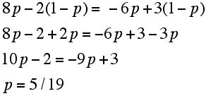
It is easily seen that q, the fraction of the time that Column should play column 1 is 9/19, though it is worth making this calculation and solving the resulting linear equation to practice how the thinking goes.
To find out who has an advantage, one can substitute the value p=5/19 into the left or right hand side of the equation above. One sees that Row's payoff is 12/19 and, thus, Column's payoff is -12/19. This is not such an easy number to see without the mathematics! Thus, if this game is repeated 19 times the payoff to Row will be approximately $12. Each time the game is played $8, $6, $3 or $2 changes hands but on the average, over a long number of plays of this game, Row will win 12/19 of a dollar on each play of the game and Column will lose 12/19 of a dollar on each play.
A famous theorem of von Neumann in essence shows that for a two-player zero-sum game where Row has m choices and Column has n choices, each time the game is played that game has an optimal mixed strategy for each player. This optimal strategy has the property that if either player deviates from the mixed strategy which is best for him/her, then that player will only do worse.
Nash Equilibria
However, many of the most interesting games that mathematicians and those who try to apply game theory in the real world have to analyze are not zero-sum games. For example the game below might be a model of the situation described earlier in which a couple is trying to decide whether to go to a movie or to the opera.
| Column 1 (Opera) | Column 2 (Movie) | |
| Row I (Opera) | (6, 2) | (4, 4) |
| Row II (Movie) | (7, 4) | (10, 3) |
Using dominating strategy analysis this game has the "solution" of Row playing row II and Column playing column 1, using pure strategies. However, other nonzero-sum games, such as the one we saw in Figure 4, do not have a solution in pure strategies. Remarkably, it has been shown that if one moves to the domain of "mixed strategies" there will always be an "equilibrium" solution for Row and Column - that there will always be a "Nash Equilibrium." The concept is named for John Nash, who won the Nobel Prize in Economics for his seminal work in showing the existence of the "equilibria" that now bear his name. Nash's Theorem is an existence theorem.

He uses mathematics, the Kakutani fixed point theorem, to show that equilibria exist for certain games but does not show how to find them. In fact, the issue of determining the number and computational complexity of finding Nash Equilibria for games is still a wide open area of research. The basic idea behind the concept of a Nash Equilibrium is that for wide classes of games there are ways for the players to play the game, sometimes as pure strategies and sometimes as mixed strategies so that if a player deviates from the Nash Equilibrium strategy, he/she can not improve his/her payoff. Our more detailed analysis of the two-person zero-sum games with two action choices for each player gives the spirit of what is involved.
Fictitious Play
For those with mathematical skill one can master the techniques for finding the optimal play of games such as the ones we have been looking at. It would be nice, however, if there was a more pragmatic approach to playing a game such as the one we solved (Figure 6). An insight into this was obtained by the mathematician Julia Robinson (1918-1985), who is much better known for her famous role in the solution of Hilbert's 10th Problem. Robinson was also the first woman President of the American Mathemtical Society. She proved an intriguing result based on an idea pioneered by the Princeton educated mathematician George William Brown. Brown introduced the idea of "fictitious play," though the terminology is not particularly felicitous because it is a technique that often can be used in practice to play games.

Suppose you are asked to play a zero-sum game with no dominating rows or columns such as the one in Figure 6. You could, if you have mastered how, do the calculations we did to find the optimal way to play. However, another approach might be to see if there was some "adaptive" way to play the game. Intuitively, the idea is to learn from playing the game to be able to play the game better. Start by making what you hope is a good first move, look at the payoff you receive based on your opponent's choice and then move in the future in a way to try to "improve" (or not make worse) your situation. What Julia Robinson showed is that for 2-person zero-sum games this "learning as you go along" approach to games works. In the end, if each player adopts this point of view they will eventually converge to their optimal mixed strategies. Unfortunately, as shown by Lloyd Shapley this is not true for all games. Shapley provided an example of a 3x3 game for which the adaptive learning approach does not work. Robinson's work and extensions of it have important connections to the area of mathematics known as dynamical systems. Robinson's work has been extended in a variety of ways. Other works have been showing connections between ideas involving adaptive approaches to playing games and learning environments in general. Other researchers are showing exciting connections to ideas in evolutionary biology, where game theory is having exciting implications.
Prisoner's Dilemma
Perhaps the most famous of all games is Prisoner's Dilemma. It deserves (and perhaps will eventually get) a column of its own. The game takes its name from a "story" to accompany the matrix of the game, that is due to Albert W. Tucker, who for many years headed the Mathematics Department at Princeton University. The story helps explain the payoffs of a 2-person nonzero-sum game with a structure that has "paradoxical" implications.

(Albert W. Tucker, courtesy of his son Alan Tucker)
The game below belongs to the Prisoner's Dilemma type of game.
| Column 1 | Column 2 | |
| Row I | (3, 3) | (0, 5) |
| Row II | (5, 0) | (1, 1) |
Figure 8
If one carries out a dominating strategy analysis of this game, one sees that the players should play row II and column 2 to achieve their "best" outcome. However, the payoff of 1 to each of Row and Column is poorer than the payoff of 3 to each of them for playing row I and column 1. This creates the paradoxical situation that rational play leads to a poorer outcome than irrational play. The situation is even more dramatic when the outcomes become negative:
| Column 1 | Column 2 | |
| Row I | (8, 8) | (-6, 20) |
| Row II | (20, -6) | (-4,-4) |
Figure 9
Game theory suggests that the "rational" way to play this game is to play row II and column 2 either when the game is played once, or when there is repeated play of this game. Yet, this seems difficult to accept if there is an outcome where on each play, instead of losing 4 units, the players can each gain 8 units. However, the game theory analysis shows that playing row I and column 1 is not "stable." Players playing this way in repeated plays of this game will always be tempted by the fact that if their opponent does not shift action simultaneously, then they can improve their own payoff while "hurting" their opponent. Thus, if Column continues to play column 1 while Row moves from row I to row II, the result will be that Row earns 20 instead of 8, while Column goes from winning 8 to losing 6. Not that this is true even though Row and Column may have signed a "binding treaty." Unfortunately, Prisoner's Dilemma is not merely an intellectual curiosity. It seems like a reasonable model for various confrontational games such as those that occur between unions and management during contract negotiations, and in the relationship between countries. In fact, the US Defense Department did research into the ways games such as Prisoner's Dilemma were played by "real people" in an attempt to understand the implications of "cold war" politics during the time of the Soviet Union.
The Centipede Game
Compared with Prisoner's Dilemma the centipede game is not that well known, but like Prisoner's Dilemma, it has been a very fertile window into gaining insight into the nature of rationality. The discrepancy between the predictions that game theory makes for the way to play the centipede game and what happens in actual practice has created a torrent of research.
The centipede game, again like Prisoner's Dilemma is actually a family of games with similar characteristics but in which the specific game variant depends on a collection of numerical parameters. Experiments using different parameters yield different results and insights into the family.
This game was developed by Robert W. Rosenthal, a mathematically trained economist. However, the name for the game is due to Kenneth Binmore.

(Courtesy of Professor Randall Ellis, Dept. of Economics, Boston University)
Sadly, Rosenthal died of a heart attack in 2002 at the relatively young age of 57. His research ranged over a variety of aspects of the interplay of game theory and economics. His work often returned to the issue of what constituted sensible or rational behavior in economic settings.
The basic idea of the centipede game involves alternating moves of two players in a game which is described in "extensive form" by a tree. In looking at the current move that a player has versus the move that his/her opponent can next make, the player sees that the current pot of outcomes gives her more income than her opponent, but on the next move the reverse will be true. A generic version of the game is shown below. The two players' names are A and B and at a given vertex (white circle) of the "decision tree" the names of the players alternate. At a particular dot, say one labeled A, which is where player A must make a decision, there are two moves that A can make. A can move either to the right (go to the next vertex to the right) where A cedes to B the decision about what to do next, or A can terminate the game by going down. Going to the right in the literature of the centipede game is often described as "pass," which means the player currently to move does not terminate the game (except for the very last decision), while the decision to go down is described as "take." The two numbers at the end of the down arrow are the payoffs to A (on the left) and B (on the right). The down (take) moves are indicated in blue to contrast them with the right (pass) moves. Usually, the game is assumed to have equal numbers of decision moves for A and for B. (This means there is an odd number of 1-valent vertices or leaves in the tree.)
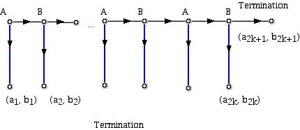
The game gets its name from the diagram above where there is a resemblance to a critter with many legs. However, consider the small version of the centipede game which is shown in Figure 11 in order to see the troublesome aspects of this game for theorists.
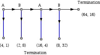
Suppose you are A. How would you play this game? Here is the mathematical reasoning that comes with treating this game as one of perfect information, where both players are completely rational each opponent behaves rationally. Suppose the game were to reach the stage where player B has to act at the far right decision vertex. Now B, preferring more money rather than less will choose take (down) at this node. This follows since if B passes, he gets 16 while his opponent A gets 64. By "taking," B gets 32 while A only gets 8. Thus, at the prior vertex, A knowing what B will do, will chose to pick take (down). Knowing this, "backward reasoning" means that at the prior node B will take, which in turn means that at the very first decision node, A should take as well! Reasoning of this kind has come to be called "backward induction." Similarly, in the "long" (e.g. many feet) version of the centipede game it means that A should choose the take (down) option on the very first play of the game. This means that both players receive relatively meager payoffs. To play longer offers each of the players a chance to make more but only at the risk that when the game is stopped, his/her opponent will walk away with more than he/she will.
In this variant of the game the amounts each player gets are going up quickly; however, in some variants, the growth is very slow. Furthermore, in some variants the initial pot, if taken, gives each equal amounts. One can look at a version of the game where the sum of the payoffs to the players is a constant. The characteristic of these games is that rational play suggests that the first player should take right at the start. Yet, this seems a perplexing choice since so much more can be gained by being "irrational." Also, note that if A passes (allows B to move) at the first node of the game, then B faces a new version of the centipede game with essentially the same structure that A had! Why might you not take at the first opportunity if you are player A? One reason is that you might have some "altruistic" component to your personality. You might also think that perhaps your opponent, if the centipede is longer (rather than having 4 legs), will make a mistake in the analysis and continue to play longer when it is his/her decision.
The situation gets interesting if one takes this game and sees what happens when real people (rather than armchair philosophers, mathematicians and game theorists) play the game! Experimental economists and other scholars have actually done this. Nearly always, real people, who have been clearly explained the rules of the game and understand them, do not terminate the game at the first move! Does this mean that the analysis of the game that we have given is wrong or does it mean that human beings are "irrational"?
Are you surprised that many people do not play this game "rationally" in the sense that when given the chance to play A at the first round, they do not choose "take"? On the other hand it is also the case that the game does not typically last as long as allowing B to make the pass move at the last vertex. Variants of the centipede game have provided a controlled environment to probe the nature of altruism, signaling to achieve cooperation, and the limits to rationality. These experiments have worked with the centipede game in extensive form as well as in recent work that gets new insights from using a normal form for the centipede game. In this work the subjects of the experiments must name the "round" where they would "take" in the centipede game rather than play the game dynamically as such. An interesting recent set of experiments concerns playing the centipede game where groups of players compete in the game against each other rather than individuals playing each other. The results here suggest that groups come closer to the prediction of "taking" on the first round of play than when individuals play. The accelerating number of papers of both a theoretical type and experimental type that draw inspiration from the centipede game are a testament to the fertility of a single game and its associated circle of ideas to stimulate mathematicians and scholars over a wide array of disciplines.
References:
Andreoni, J. and J. Miller, Rational cooperation in the finitely repeated prisoner's dilemma: experimental evidence, The Economic Journal, 103 (1993) 570-585.
Aumann, R., On the centipede game, Games and Economic Behavior 23 (1998) 97-105.
Aumann, R., Backward induction and common knowledge of rationality, Games and Economic Behavior 8 (1995) 6-19.
Aumann, R., Reply to Binmore, Games and Economic Behavior 17 (1996) 138-146.
Axelrod, R., The Evolution of Cooperation, Basic Books, New York, 1984.
Binmore, K., Modelling rational players (Part I), Economics and Philosophy, 3 (1987) 179-214,
Binmore, K., Essays on the Foundations of Game Theory, Basil Blackwell, Oxford, 1990.
Binmore, K., Fun and Games, D.C. Heath, Lexington, 1992.
Binmore, K., A note on backward induction, Games and Economic Behavior 17 (1996) 135-137.
Bornstein, G. and T. Kugler, A. Ziegelmeyer, Individual and group decisions in the centipede game: Are groups more "rational" players?, J. of Experimental Social Psychology, 40 (2004) 599-605.
Broome, J. and W. Rabinowicz, Backwards induction in the centipede game, Analysis, 59 (1999) 237-242.
Brown , G., Interactive solutions to games by fictitious play, In "Activity Analysis of Production and Allocation," T. Koopmans (ed.), Wiley, New York, 1951, p. 374-376.
Cox, J. Trust, reciprocity, and other-regarding preferences: Groups vs. individuals and males vs. females. In R. Zwick and A Rapaport (eds.) Advances in Experimental Business Research, Kluwer, Dordrecht, 2002.
Fey, M. and R. McKelvey, T. Palfrey, An experimental study of constant sum centipede game, International J. of Game Theory, 25 (1996) 269-287.
Foster, D. and R. Vohra, Calibrated learning and correlated equilibrium, Games and Economic Behavior, 21 (1997) 40-55.
Foster, D. and H. Young, Stochastic evolutional game dynamics, Theoretical Population Biology, 38 (1990) 219-232.
Foster,D. and H. Young, On the impossibility of predicting the behavior of rational agents, Proceedings of the National Academy of Sciences, 98 (2001) 12848-53.
Foster, D. and H. Young, Learning, hypothesis testing, and Nash equilibria, Games and Economic Behavior, 45 (2003) 73-96.
Fudenberg, D. and D. Levine, Consistency and cautious fictitious play, J. Econ. Dynam. Control, 23 (1995) 1605-1632.
Fudenberg, D. and D. Levine, The Theory of Learning in Games, MIT Press, Cambridge, 1998.
Gale, D. and R. Rosenthal, Experimentation, imitation, and stochastic stability, J. Economic Theory, 83 (1999) 1-40.
Gale, D. and R. Rosenthal, Experimentation, imitation, and stochastic stability: addendum, J. Economic Theory, 97 (2001) 164-174.
Goeree, J. and C. Holt, Ten little treasures of game theory and ten intuitive contradictions, American Economic Review, 91 (2001) 1402-1422.
Hart, S. and A. Mas-Colell, Uncoupled dynamics do not lead to Nash equilibria, American Economic Review, 93 (2003) 1830-1836.
Heifetz, A. and A. Pauzner, Backward induction with players who doubt others' faultlessness, Mathematical Social Sciences, 50 (2005) 252-267.
Johannsson, M. and M Palme, Idealisation and the Centipede: What is the significance of the backward induction theorem? (preprint) Department of Philosophy, Lund University, Sweden.
Kreps, D. and P. Milgrom, J. Roberts, R. Wilson, Rational cooperation in the finitely repeated Prisoners' Dilemma, J. Economic Theory 27 (1982) 245-252.
Kreps, D., Game Theory and Economic Modeling, Oxford U. Press, Oxford, 1990.
Kreps, D., A Course in Microeconomic Theory, Princeton U. Press, Princeton, 1990.
Kuhn, H., (ed.), Classics in Game Theory, Princeton U. Press, Princeton, 1997.
Luce, R. and H. Raiffa, Games and Decisions, Wiley, New York 1957.
Macrae, N., John Von Neumann, Pantheon Books, New York, 1992.
McKelvey, R. and T. Palfrey, An experimental study of the centipede game, Science Working Paper 732, California Institute of Technology, 1990.
McKelvey, R. and T. Palfrey, An experimental study of the centipede game, Econometrica 60 (1992) 803-836.
McKelvey, R. and T. Palfrey, A statistical theory of equilibrium in games, Japanese Econom. Review 47 (1996) 186-209.
Nagel, R. and F. Tang, Experimental results on the centipede game in normal form: An investigation on learning, J. of Mathematical Psychology, 42 (1988) 356-384.
Neumann, J. von, and O. Morgenstern, Theory of Games and Economic Behavior, Princeton U. Press, Princeton, 1944.
Ponti, G., Cycles of learning in the centipede game, Games and Economic Behavior 30 (2000) 115-141.
Poundstone, W., Prisoner's Dilemma, Doubleday, New York, 1992.
Rabinowicz, W., Grappling with the centipede: Defense of backward induction for biterminating games, Economics and Philosophy, 14 (1998) 95-126.
Radner, R. and D. Ray, Robert W. Rosenthal, J. of Economic Theory, 112 (2003) 365-368.
Rapoport, A., Games Fights, and Debates, U. Michigan Press, Ann Arbor, 1961.
Rapoport, A., (ed.) Game Theory as a Theory of Conflict Resolution, D. Reidel, Boston, 1974.
Rapoport, A. and A. Chammah, Prisoner's Dilemma, U. Michigan Press, Ann Arbor, 1965.
Rapoport, A. and M. Guyer, D. Gordon, The 2x2 Game, U. Michigan Press, Ann Arbor, 1976.
Rapoport, A. and W. Stein, J. Parco, T. Nicholas, Equilibrium play and adaptive learning in a three-person centipede game, Games and Economic Behavior 43 (2003) 239-265.
Robinson, J., An iterative method of solving a game, Annals of Mathematics, 54 (1951) 296-301.
Rosenthal, R., Sequences of games with varying opponents, Econometrica, 47 (1979) 1353-1366.
Rosenthal, R., Games of perfect information, predatory pricing and the chain store paradox, J. Ecomic Theory 25 (1981) 92-100.
Rosenthal, R. and H. Landau, A Game-Theoretic Analysis of Bargaining with Reputations, J. Math. Psych., 20 (1979) 233-255.
Roth, A., Axiomatic Models of Bargaining, Springer-Verlag. Berlin, 1979.
Selten, R., Reexamination of the perfectness concept for equilibrium points in extensive form games, International J. of Game Theory, 4 (1982) 25-55.
Sobel, H. Backward induction arguments in finitely iterated prisoners' dilemmas: a paradox regained, Philosophy of Science, 60 (1993) 114-133.
Weintraub, E., (ed.), Toward a History of Game Theory, Duke University Press, Durham, 1992.
Young, H., Strategic Learning and Its Limits, Oxford U. Press, Oxford, 2004.
Zauner, K., A payoff uncertainty explanation of results in the experimental centipede games, Games and Economic Behavior 26 (1999) 157-185.
NOTE: Those who can access JSTOR can find some of the papers mentioned above there. For those with access, the American Mathematical Society's MathSciNet can be used to get additional bibliographic information and reviews of some these materials. Some of the items above can be accessed via the ACM Portal, which also provides bibliographic services.
Joseph Malkevitch
York College (CUNY)
malkevitch at york.cuny.edu ![]()


No comments:
Post a Comment